It's always best to perform practical implementation to better understand a concept. In this section, we'll be executing a small demo that will show you how to calculate the Mean, Median, Mode, Variance, Standard Deviation and how to study the variables by plotting a histogram. This is quite a simple demo but it also forms the foundation that every Machine Learning algorithm is built upon.

Step 1: Import data for computation

>set.seed(1)

#Generate random numbers and store it in a variable called data

>data = runif(20,1,10)

Step 2: Calculate Mean for the data

#Calculate Mean

>mean = mean(data)

>print(mean)

[1] 5.996504

Step 3: Calculate the Median for the data

#Calculate Median

>median = median(data)

>print(median)

[1] 6.408853

Step 4: Calculate Mode for the data

#Create a function for calculating Mode

>mode <- function(x) { >ux <- unique(x) >ux[which.max(tabulate(match(x, ux)))]

}

>result <- mode(data) >print(data)

[1] 3.389578 4.349115 6.155680 9.173870 2.815137 9.085507 9.502077 6.947180 6.662026

[10] 1.556076 2.853771 2.589011 7.183206 4.456933 7.928573 5.479293 7.458567 9.927155

[19] 4.420317 7.997007

>cat("mode= {}", result)

mode= {} 3.389578

Step 5: Calculate Variance & Std Deviation for the data

#Calculate Variance and std Deviation

>variance = var(data)

>standardDeviation = sqrt(var(data))

>print(standardDeviation)

[1] 2.575061

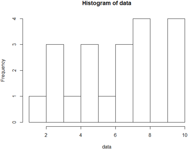
Step 6: Plot a Histogram

#Plot Histogram

>hist(data, bins=10, range= c(0,10), edgecolor='black')

The Histogram is used to display the frequency of data points: