In this demo, we'll be using the gapminder data set to perform hypothesis testing. The gapminder data set contains a list of 142 countries, with their respective values for life expectancy, GDP per capita, and population, every five years, from 1952 to 2007.

We'll begin by downloading the gapminder package and loading it into our R environment:

#Install and Load gapminder package

install.packages("gapminder")

library(gapminder)

data("gapminder")

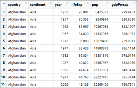
Now, let's take a look at our data set by using the View() function in R:

#Display gapminder dataset

View(gapminder)

Here's a quick look at our data set:

The next step is to load the infamous dplyr package provided by R. We're specifically looking to use the pipe (%>%) operator in the dplyr package. For those of you who don't know what the pipe operator does, it basically allows you to pipe your data from the left-hand side into the data at the right-hand side of the pipe. It's quite self-explanatory.

#Install and Load dplyr package
install.packages("dplyr")
library(dplyr)
Our next step is to compare the life expectancy of two places (Ireland and South Africa) and perform the t-test to check if the comparison follows a Null Hypothesis or an Alternate Hypothesis.

#Comparing the variance in life expectancy in South Africa & Ireland
df1 <-gapminder %>%
select(country, lifeExp) %>%
filter(country == "South Africa" | country =="Ireland")
So, after you apply the t-test to the data frame (df1), and compare the life expectancy, you can see the below results:

#Perform t-test

t.test(data = df1, lifeExp ~ country)

Welch Two Sample t-test

data: lifeExp by country
t = 10.067, df = 19.109, p-value = 4.466e-09
alternative hypothesis: true difference in means is not equal to 0
95 percent confidence interval:
15.07022 22.97794
sample estimates:
mean in group Ireland mean in group South Africa
73.01725 53.99317
Notice the mean in group Ireland and in South Africa, you can see that life expectancy almost differs by a scale of 20. Now we need to check if this difference in the value of life expectancy in South Africa and Ireland is actually valid and not just by pure chance. For this reason, the t-test is carried out.

Pay special attention to the p-value also known as the probability value. p-value is a very important measurement when it comes to ensuring the significance of a model. A model is said to be statistically significant only when the p-value is less than the pre-determined statistical significance level, which is ideally 0.05. As you can see from the output, the p value is 4.466e-09 which is an extremely small value.In the summary of the model, notice another important parameter called the t-value. A larger t-value suggests that the alternate hypothesis is true and that the difference in life expectancy is not equal to zero by pure luck. Hence in our case, the null hypothesis is disapproved.

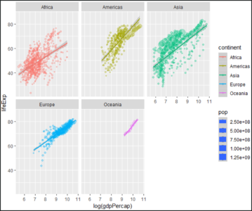
To conclude the demo, we'll be plotting a graph for each continent, such that the graph shows how the life expectancy for each continent varies with the respective GDP per capita for that continent.

#Plotting a gdpPercap vs lifeExp graph for each continent
#Install and Load ggplot2 package
install.packages("ggplot2")
library(ggplot2)
gapminder%>%
filter(gdpPercap < 50000) %>%
ggplot(aes(x=log(gdpPercap), y=lifeExp, col=continent, size=pop))+
geom_point(alpha=0.3)+
geom_smooth(method = lm)+
facet_wrap(~continent)